Excel offers many text functions that are super helpful if you need to edit or make additions to your text strings. In this tutorial I’ll teach you how to use them.
Joining strings in Excel
If you want to join two different text string you can use the & operator.
1. Select the cells where you want to join strings and insert the & operator.
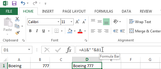
To join cells A1 and B1 the Text function would look like this:
=A1&B1
Note that to insert an additional character (such as a space) you have to use the ” ” operator.
To join cells A1 and B1 the Text function would look like this:
=A1&" "&B1
Using the LEFT Function
If you want to get just a specific amount characters on the left of a string then the LEFT function is a very helpful tool.
1. Insert the LEFT function.
2. Select the cell where you want to extract the leftmost characters from and specify how many characters you want to extract.
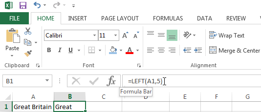
If you want to extract the first 5 characters from your string in cell A1 then your LEFT function would look like this:
=LEFT(A1, 5)
Using the RIGHT Function
If you want to get just a specific amount characters on the right of a string then you should use the RIGHT function.
1. Insert the RIGHT function.
2. Select the cell where you want to extract the rightmost characters from and specify how many characters you want to extract.
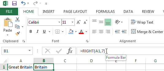
If you want to extract the last 7 characters from your string in cell A1 then your RIGHT function would look like this:
=Right(A1, 7)
Using the MID function
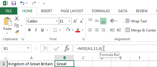
Use the MID function to extract a substring of a specific string, starting from a character you specify by number and up to an amount you specify after.
In the example below, I use =MID(A1,11,6) to extract text at position 11 (G), and extracted 6 characters (Great). Also note that Excel counts spaces as a position.
Using the LEN function
If you want to find out the length of a string then the LEN function is super useful.
1. Insert the LEN function.
2. Select the cell where you want to know the length of the string.
If you want to find out the length of the string in cell A1 then your LEN function would look like this:
=LEN(A1)
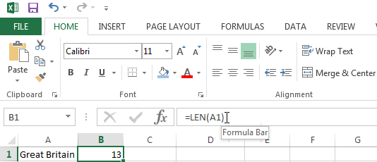
Note that the value includes special characters such as a space.
Using the FIND function
If you want to find the position of a substring then the FIND function is very helpful.
1. Insert the FIND function.
2. Write the characters (substring) you are looking for in your string and the cell where you want Excel to look.
If you want to find the location of “Great” in cell A1 then your function would look like this:
=FIND("Great", A1)
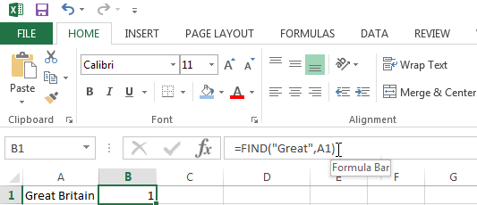
Note how Excel found string “Great” at position 1.
Using the SUBSTITUTE function
If you want to replace a certain substring of your text with a new substring the SUBSTITUTE function is an excellent tool.
1. Insert the SUBSTITUTE function.
2. Select the cell where the string of text you want to replace is.
3. Then write the old text in quotes, and the new text you want it to be substituted with.
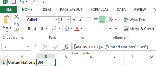
For example: If you want the string “United Nations” in cell A1 to be replaced with “UN” then your substitute function would look like this:
=SUBSTITUTE(A1,"United Nations","UN")
A pretty long lesson this one, but trust me you’re going to use these functions a lot in your Excel work.
If you have any questions, just let me know below in the comments. I read them all and will answer you personally.

i want to separate word in a excel ‘Allowences. This i need to remove first ‘ (symbol) from each word in the list. pls tell me how to do this……
use Subtitute in Formulas, in the field “old text” fill (‘) symbol